A Matter of Opinion

The Capital Asset Pricing Model, or CAPM, remains the most influential model in finance, largely due to its elegant structure and powerful conclusions. The main conclusions of the CAPM are 1) all investors hold the market portfolio in combination with a risk-free asset (long or short) making optimization unnecessary and 2) the expected return in excess of the risk-free rate of each security is proportional to its systematic risk with respect to the market portfolio (beta). These conclusions, however, depend heavily on the assumptions of the model. Changing the assumptions leads to very different conclusions. In previous issues of Quant U, I showed what happens when we separately relax or change three of the CAPM's assumptions:1

1. The standard CAPM assumes investors only care about the expected return and risk as measured by the standard deviation of the returns on their portfolios. In "The Popularity Asset Pricing Model" (June/July 2018), I relaxed this assumption to allow for investor preferences regarding characteristics other than expected return and standard deviation, thus forming the Popularity Asset Pricing Model, or PAPM. The conclusions: Each investor holds a portfolio tailored to reflect his or her preferences arrived at via an optimization, and the expected excess return on each security depends not only on beta but also on exposure to the other characteristics that investors care about.
2. The standard CAPM assumes investors are free to take short positions in any security. In "What Harry Markowitz Doesn't Like About the CAPM" (Summer 2019), I presented an example developed by Markowitz (2015) to show what happens if investors cannot short. In this case, portfolios are often investor-specific because it may not be possible to short some securities. Somewhat surprisingly, there is no relationship between expected return and beta.
3. The standard CAPM assumes there is a riskless security, which an investor can hold or short. In "Why the CAPM Falls Flat" (Fall 2019), I presented a version of the CAPM called the Black CAPM or the Zero-Beta CAPM, developed by Black (1972). In this version of the CAPM, there is no riskless security. In this model, each investor selects a portfolio on the efficient frontier based on his or her level of risk aversion. Therefore, portfolios are investor specific. Also, while there is a linear relationship between beta and expected return, the line plotting beta versus expected return can be flatter than it is in the standard CAPM. Hence, securities with high betas have lower expected return than predicted by the standard CAPM, and securities with low beta have higher expected returns than predicted by the standard CAPM.

In this issue of Quant U, I explore the consequences of relaxing a fourth key assumption: that all investors hold the same, correct beliefs about expected returns, standard deviations of returns, and correlations of returns. Instead, I assume that each investor holds his or her own opinion of the expected return on each security. In a recent working paper,2 Thomas Idzorek, Roger Ibbotson, and I make this assumption to generalize both the CAPM and the PAPM as described by Ibbotson et al. (2018).3 While this approach is not new (it was first taken by Lintner 1969), it is not common among those trying to develop better asset-pricing models, at least in the form that we used in our paper. As with the other cases of relaxing or changing a key assumption, our conclusions are quite different from those of the standard CAPM.

In our working paper, we present generalized versions of the CAPM and PAPM in two ways: 1) as formal mathematical models and 2) using a numerical example. Here, I present the numerical model to illustrate what happens when investors hold different opinions about expected returns on different securities.

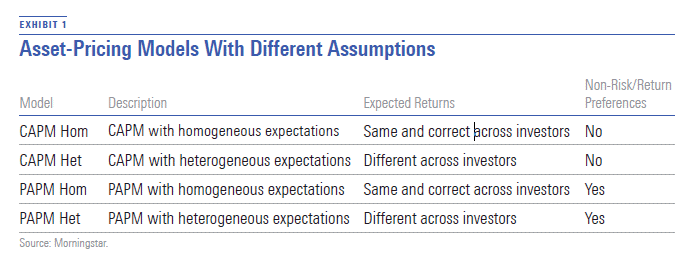
A Numerical Example We illustrate the consequences of investors holding different opinions on expected returns by constructing the four models described in Exhibit 1 from the same set of parameters.

- source: Morningstar Analysts

Hom

is short for

homogeneous

expectations, in which all investors have the same expectations.

Het

is short for

heterogeneous

expectations, in which investors have differences in expectations. CAPM Hom is the standard CAPM. All investors hold the same and correct views of expected returns. PAPM Hom is the model described in our working paper.

In our paper, we illustrate the four models described in Exhibit 1 using a set of parameters on six securities (A, B, C, D, E, and F), with two non-risk/return popularity characteristics (X and Y), and six investors (1, 2, 3, 4, 5, and 6). The example is designed in the spirit of a controlled experiment to highlight the incremental differences in the various models, isolating the effects of risk aversion, forecasting skill, and popularity preferences on expected returns and security prices.

Some notes about our example:

• Security A is the only high-risk security; Security B is the only low-risk security. The other four securities all have moderate risk.
• Investor 1 is the only investor with a low level of risk aversion; Investor 2 is the only investor with a high level of risk aversion. The other four investors all have moderate risk aversion.
• Security E is the only security that exhibits popularity Characteristic X, and Investor 5 is the only investor who prefers Characteristic X. This preference is strongly positive.
• Security F is the only security that exhibits popularity Characteristic Y. Investor 6 is the only investor who prefers Characteristic Y. This preference is strongly negative.

Exhibit 2 compares the expected returns of each security under the CAPM Hom and the PAPM Het models.

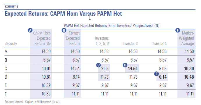
1. In the second column, Exhibit 2 shows the expected returns of all investors under the CAPM Hom model for each security. Remember, under the CAPM Hom model, all investors hold the same, correct beliefs about expected returns and have no preferences other than preferring higher expected returns to lower expected returns and lower risk to higher risk.
2. In the third column, Exhibit 2 shows the correct expected return of each security under the PAPM Het model. These expected returns may or may not be known to the individual investors depending on their levels of skill with respect to each security. Next, we turn to the forecasts of the investors individually and see whether their forecasts are correct. Investors 1, 2, 5, and 6 have the same views on expected returns of each security.
3. They are correct for every security except C and D. In other words, these investors have perfect skill regarding securities A, B, E, and F.
4. Investor 3 has the highest view on the expected return of Security C (14.54%) and is correct.
5. Investor 4 has the lowest opinion on the expected return on Security D (6.14%) and is correct. Investor 3 has perfect skill regarding Security C, and Investor 4 has perfect skill regarding Security D. All of the investors hold views on all other securities (A, B, E, and F) that are correct.
6. Finally, we look at the market-weighted average opinion of expected returns. These are correct for Securities A, B, E, and F. They are incorrect for Securities C and D due to the forecasting errors of every investor except for Investor 3 for Security C and of every investor except for Investor 4 for Security D.

Exhibit 3 shows the weights of the market portfolio under the CAPM with homogeneous expectations and the portfolio of each of the six investors under the PAPM with heterogeneous expectations.

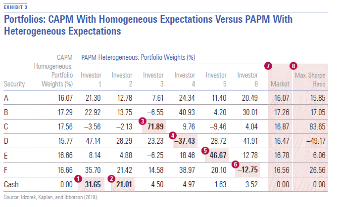
1. Investor 1 shorts the risk-free asset (cash) to create a levered portfolio based on his low level of risk aversion.
2. Investor 2 invests part of her wealth in the risk-free asset to create an unlevered portfolio based on her high level of risk aversion.
3. Investor 3's large allocation to Security C is due to his correct high level of the expected return on Security C (as we saw in Exhibit 2).
4. Investor 4's large short position in Security D is due to her correct low level of the expected return on Security D.
5. Investor 5's large allocation to Security E is due to his strong preference for its exposure to Characteristic X.
6. Investor 6's short position in Security F is due to her strong negative preference for its exposure to Characteristic Y.
7. The market portfolio under the PAPM with heterogeneous expectations is the aggregation of the portfolios of all market participants. In general, this is not on the efficient frontier drawn using correct expectations. (More on this later.)
8. The portfolio under the PAPM Het that maximizes the Sharpe ratio is on the efficient frontier drawn using correct expectations.4 (Again, more on this later.)

Plotting Risk and Expected Return Exhibits 4 through 7 show the expected returns and standard deviation of the securities and the investor portfolios under each of the four models (CAPM Hom, CAPM Het, PAPM Hom, and PAPM Het).

All of the points shown in these four exhibits are plotted using correct expectations. In addition to the points representing the securities and investor portfolios, each exhibit includes:

• The efficient frontier of risky securities.
• The market portfolio.
• The portfolio that maximizes the Sharpe ratio.
• The capital market line; i.e., the line that runs through the risk-free asset and that is tangent to the efficient frontier at the portfolio that maximizes the Sharpe ratio.

There are important and subtle differences across the four charts.

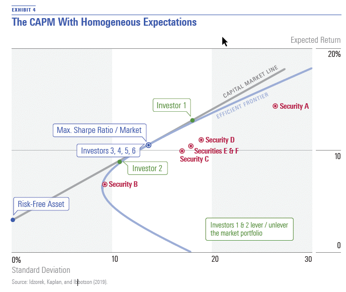
We start with the CAPM Hom model in Exhibit 4. Here, the market portfolio and Sharperatio- maximizing portfolio are one and the same. Because Investors 3, 4, 5, and 6 each have the same moderate level of risk aversion as the market average level of risk aversion, they all hold the market/Sharpe-ratio-maximizing portfolio. Investor 1 has lower-than-average risk aversion and chooses a levered position in the market portfolio. Investor 2 has higher-thanaverage risk aversion and chooses an unlevered position in the market portfolio.

Looking across Exhibits 5, 6, and 7, the risk and expected return of at least two securities are different relative to what Exhibit 4 shows; as such, each of the corresponding efficient frontiers is different. The three efficient frontiers result in Sharpe-ratio-maximizing portfolios that no longer correspond with the original market portfolio nor the corresponding market portfolio in a given model. This leads to three distinct capital market lines, all of which dominate the corresponding market portfolio and show that the market portfolio is not efficient when one incorporates either unique forecasts or popularity preferences. (In the case of PAPM Hom, which is shown in Exhibit 6, the plot point of the market portfolio turns out to be very close to the plot point of the Sharpe-ratiomaximizing portfolio, making it difficult to tell visually that it is beneath the tangency line.)

Exhibit 5 shows the CAPM Het model. We see that all six of the investors are making at least one forecasting error, creating portfolios that aren’t optimal. Investors 1, 2, 5, and 6 have the same correct estimates of expected returns for Securities A, B, E, and F, but they all have estimated the wrong expected returns for both Securities C and D. Investor 3 is the only investor who recognizes Security C is underpriced, and Investor 4 is the only investor who recognizes Security D is overpriced—they are more skilled and their portfolios are closer to the efficient frontier.

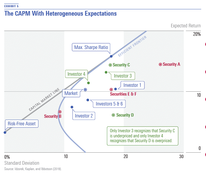
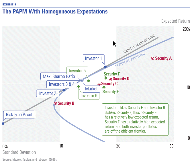
Exhibit 6 shows the PAPM Hom, Investors 5 and 6 have distinct preferences for the Characteristics X and Y exhibited by Securities E and F, respectively, which cause them to no longer hold the market portfolio. Instead, they form unique portfolios reflecting their preferences, resulting in an equilibrium that differs from that of the standard CAPM. Notice that the plot points of Securities E and F differ from what they are in Exhibit 4. Investor 5 and 6 arrive at unique portfolios, and Investors 1, 2, 3, and 4 find the Sharpe-ratiomaximizing portfolio that Investor 1 levers and Investor 2 unlevers.

Finally, in Exhibit 7, which shows the PAPM Het, we can see the combined effects of heterogeneous expectations and popularity preferences simultaneously—that is, the unique expected returns of Investors 3 and 4 for Securities C and D, as well as the preferences of Investors 5 and 6 for Securities E and F. Securities C, D, E, and F all have plots points that differ from what they are in the standard CAPM (Exhibit 4), and no investor holds portfolios on the capital market line.

More Realistic Assumptions The original CAPM and PAPM models with homogeneous expectations have very similar assumptions, yet due to the PAPM's ability to consider investor preferences beyond risk and return, the two models lead to very different conclusions. Under the CAPM, the market portfolio is the Sharpe-ratio-maximizing portfolio. Under the PAPM, it is not. Likewise, under the CAPM, mean-variance optimization is not necessary to arrive at an investor's ideal portfolio, but under the PAPM, it is. Finally, under the CAPM, the expected excess return of each security is proportional to its systematic risk with respect to the market portfolio. Under the PAPM, it is not.

Relaxing the CAPM assumption that all investors share the same heterogeneous forecasts leads to investors arriving at unique portfolios that reflect their own unique forecasts. This is vastly different from the standard CAPM world, in which all investors hold a portion of their wealth in the market portfolio. Relaxing the same assumption for the PAPM has no major impact on the conclusions of the model—only that the rationale for holding a unique portfolio is expanded beyond unique preferences to include unique forecasts. To put it bluntly, most of the elegance and ease of the CAPM falls apart when we allow heterogeneous forecasts, while the PAPM is nearly unaffected.

For both the CAPM and the PAPM, allowing heterogeneous forecasts means that not all investors have correct forecasts, making the market less than perfectly efficient. Finally, the PAPM with heterogeneous expectations can be viewed as an extension of the standard CAPM, but it may be more useful to view the CAPM as a special case of the PAPM Het. By incorporating investor preferences and allowing for heterogeneous forecasts, the PAPM Het takes two major steps toward realistic asset-pricing assumptions.

References Black, F. 1972. "Capital Market Equilibrium with Restricted Borrowing." Journal of Business, Vol. 45, No. 3 (July), PP. 444–455.

Ibbotson, R.G., Idzorek, T.M., Kaplan, P.D., & Xiong, J.X. 2018. Popularity: A Bridge Between Classical and Behavioral Research. CFA Institute Research Foundation.

Idzorek, T.M., Kaplan, P.D., & Ibbotson, R.G. 2019. “The PAPM With Heterogeneous Preferences and Expectations.” Working paper, August.

Lintner, J. 1969. “The Aggregation of Investor’s Diverse Judgments and Preferences in Purely Competitive Security Markets.” Journal of Financial and Quantitative Analysis, 4 (4), PP. 347–400.

Markowitz, H.M. 2005. “Market Efficiency: A Theoretical Distinction and So What?” Financial Analysts Journal, Vol. 61, Issue 5 (September/October), PP. 17–30.

1 In each case, all of the remaining assumptions of the standard CAPM hold. 2 Idzorek, Kaplan, and Ibbotson (2019). 3 In these models, the standard CAPM assumptions of unlimited borrowing and lending at the same riskless rate and unlimited short selling hold. 4 The Sharpe ratio is the ratio of expected excess return (expected return minus the riskless rate) to standard deviation. Under CAPM Hom, the market portfolio is the portfolio that maximizes the Sharpe ratio. In other models, the market portfolio and the portfolio that maximizes the Sharpe ratio differ.

This article originally appeared in the Winter 2019 issue of Morningstar magazine. To learn more about Morningstar magazine, please visit our corporate website.