Why the CAPM Falls Flat

This article originally appeared in the fall 2019 issue of Morningstar Magazine. To learn more about Morningstar Magazine, please visit our corporate website.

The Capital Asset Pricing Model is one of the most influential models in finance. It makes strong assumptions about investor behavior from which it derives strong conclusions about portfolio construction and expected returns. Its assumptions are:

• A1 Transaction costs and other illiquidities can be ignored.
• A2 All investors hold mean-variance efficient portfolios.
• A3 All investors hold the same (correct) beliefs about means, variances, and correlations of returns of securities.
• A4 Every investor can lend all she or he has or can borrow all she or he wants at the risk-free rate.
• A4' Investors can sell short without limit and use the proceeds of the sale to buy long positions.

Its two main conclusions are:

• C1 Each investor holds the market portfolio of risk assets in combination with a risk-free asset (long or short).
• C2 The expected return in excess of the risk-free return on each security is the security's systematic risk with respect to the market portfolio (beta) times the expected excess return on the market portfolio.

In the Summer 2019 issue of Quant U, I discussed how Harry Markowitz, the father of portfolio theory, showed that the conclusions of the CAPM do not hold if assumption A4' is violated.

Here, I discuss an alternative version of the CAPM in which A4 does not hold, leading to different conclusions. This version of the CAPM was developed by the late Fischer Black (1972)[1], so it is sometimes called the Black CAPM. For reasons that will become evident in my discussion here, it is also called the Zero-Beta CAPM.

A 3-Security Example In the previous Quant U, I illustrated the impact of dropping A4' with a three-security example. Here, I demonstrate the impact of dropping A4 with another three-security example. In the example here, two of the securities (Security A and Security B) are risky securities with expected returns and standard deviation of returns shown in Exhibit 1. The third security is the risk-free asset. As Exhibit 1 shows, the risk-free asset has a return of 3% and standard deviation of returns of zero.

Because there are only two risky securities, the efficient frontier of risky securities consists entirely of combinations of them. The curve in Exhibit 1 represents all combinations of Security A and Security B, starting with negative 20% in Security A and 120% in Security B at the upper part of the curve and ending with 130% in Security A and negative 30% in Security B at the lower part of the curve. The minimum variance portfolio, labeled "Min. Var. Port.," is at about 86% in Security A and 14% in Security B. Points along the curve above the minimum variance portfolio constitute the efficient frontier. This is why I made the part of the curve above the minimum variance portfolio solid and the part below it dotted.

In the standard CAPM, there is a risk-free asset that investors can combine with risky assets to form their portfolios. In this scenario, the risky securities should be combined into a portfolio to maximize the Sharpe ratio, which is defined as follows:

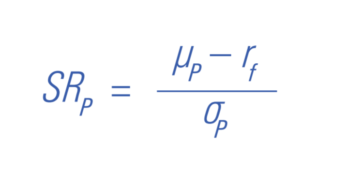
where:

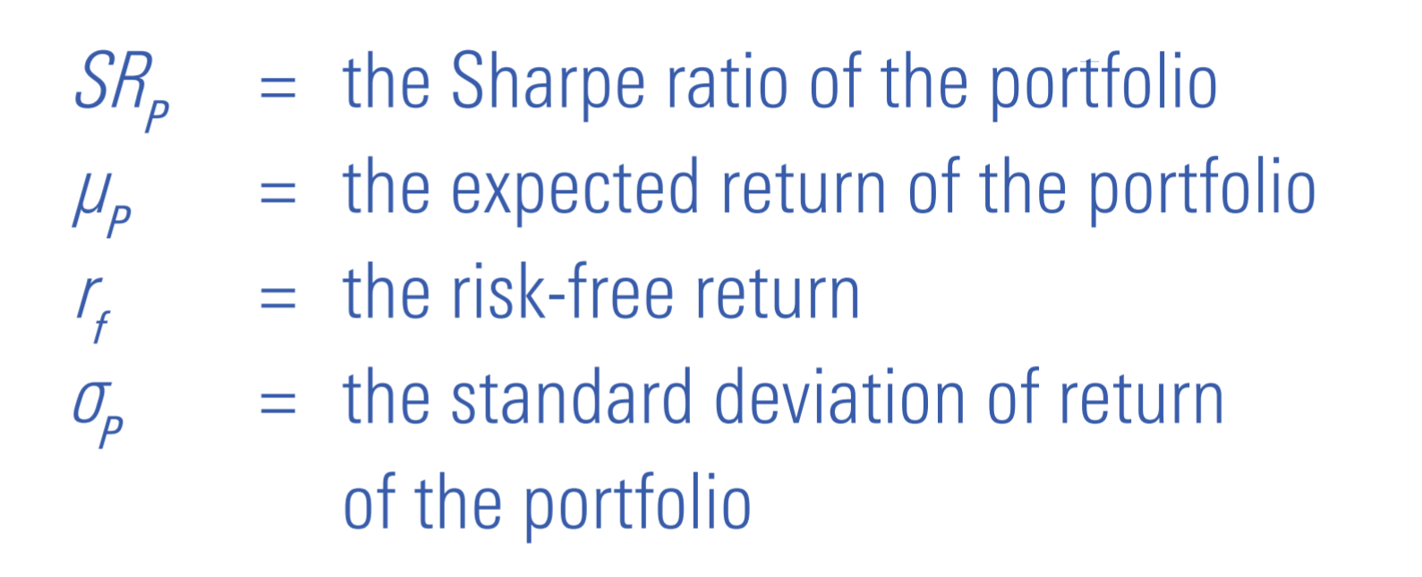
Exhibit 1 shows how to locate the portfolio that maximizes the Sharpe ratio graphically. If, from the point representing the risk-free asset, we draw a line that is tangent to the efficient frontier curve, the point of tangency is the portfolio that maximizes the Sharpe ratio. In the example here, this portfolio, which is labeled "Max. Sharpe Ratio," is about 64% in Security A and 36% in Security B.

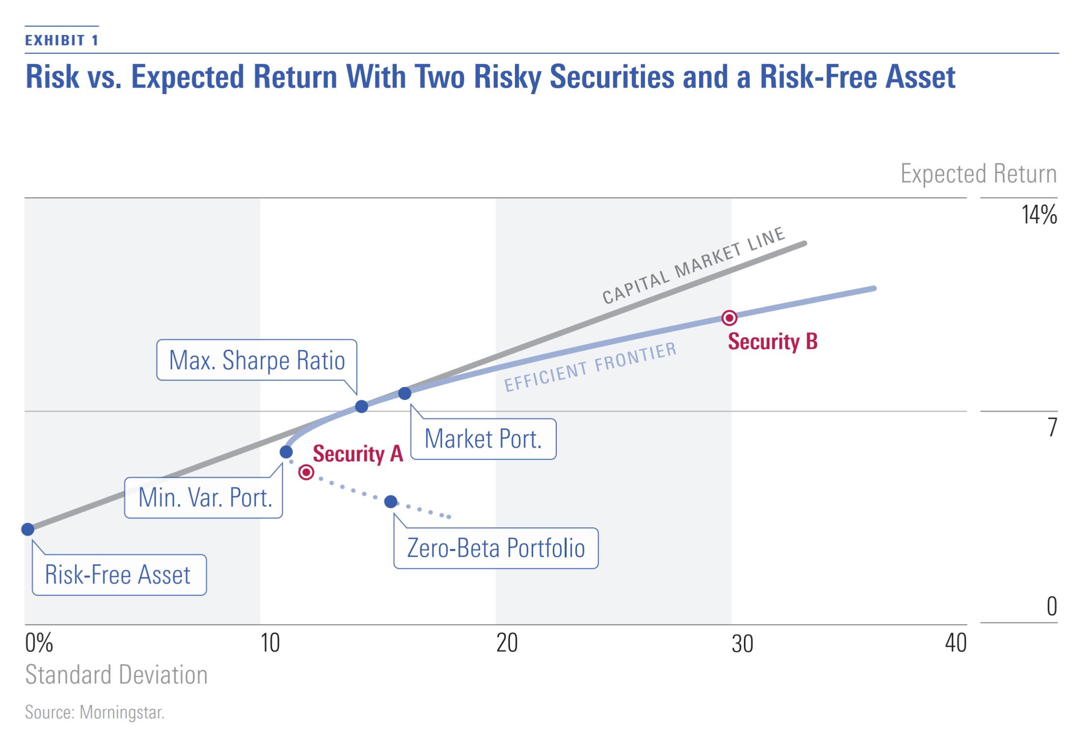
In the standard CAPM, because all investors can borrow or lend at the same risk-free rate, all investors hold some combination of the portfolio of risky securities that maximizes the Sharpe ratio and the risk-free asset (long or short); in this way, they maximize the Sharpe ratio of their portfolios at the desired risk levels. In other words, all investors hold portfolios along the tangent line rather than the efficient frontier of risky securities. This makes the portfolio that maximizes the Sharpe ratio the market portfolio.

In contrast, in the Black CAPM—in which investors cannot borrow or lend at the risk-free rate—investors are limited to portfolios on the efficient frontier of risk assets. Each investor can hold a different portfolio, thus violating conclusion C1. The market portfolio is just the wealth-weighted average of the investors' portfolios. (In the example, I assumed that this is 50% in Security A and 50% in Security B.) As I discuss below, when the market portfolio is not the portfolio that maximizes the Sharpe ratio, conclusion C2 does not hold, and a different relationship between expected return and systematic risk emerges. To state the relationship between systematic risk and expected return, we need to introduce a portfolio of risky assets that has zero systematic risk with respect to the market portfolio. Because such a portfolio has a beta of zero, it is called the Zero-Beta Portfolio. In the example in Exhibit 1, the Zero-Beta Portfolio is about 119% in Security A and negative 19% in Security B. It is on the frontier curve, but below the mean variance portfolio, so it is not a portfolio any investor would hold.

Exhibit 2 shows the allocations that the various points in Exhibit 1 represent. Each corner of the triangle represents a 100% allocation to the security indicated by the label: Security A, Security B, and the risk-free asset. Each point on a side of the triangle represents a portfolio of the two securities at the corners that the side connects, with a 0% allocation to the security at the remaining corner. Each point inside of the triangle represents a portfolio in which all three securities are held long. Points outside of the triangle represent portfolios that contain short positions.

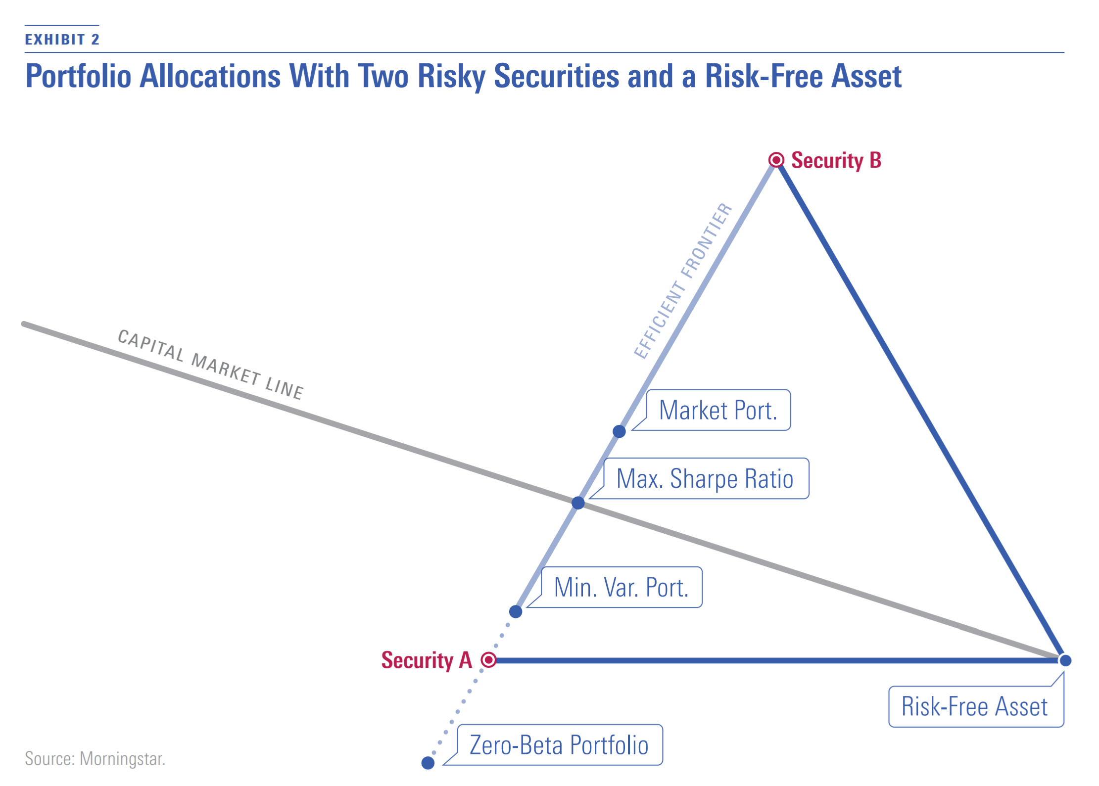
In Exhibit 2, the efficient frontier of risky securities runs along the line connecting Security A and Security B above the point representing the minimum variance portfolio. The portfolio that maximizes the Sharpe ratio and the market portfolio is on the efficient frontier. The Zero-Beta Portfolio lies on the dotted line representing inefficient portfolios of risky securities.

If investing in the risk-free asset were an option, all investors would hold the portfolio that maximizes the Sharpe ratio together with the risk-free asset in some combination. In Exhibit 2, these combinations are represented by the line labeled "Capital Market Line," which starts at a 100% allocation to the risk-free asset and passes through the portfolio that maximizes the Sharpe ratio.

Beta and Expected Returns In the standard CAPM, the expected return on any security or portfolio (μP) is related to the risk-free rate (rf), the expected return on the market portfolio (μM), and the security or portfolio beta (P) as follows:

In Exhibit 3, the line labeled "Standard CAPM" depicts this relationship using the assumptions of the example that I present here. In the standard CAPM, this line is called the security market line.

Black (1972) showed that when there is no risk-free asset, the risk-free rate is replaced by the expected return of the Zero-Beta Portfolio (μZ):

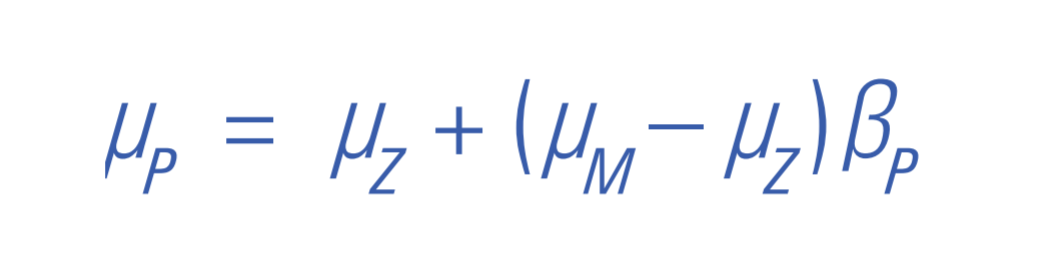
In Exhibit 3, the line labeled "Zero-Beta CAPM" depicts this relationship using the assumptions of the example that I present here. It is an alternative to the security market line of the standard CAPM.

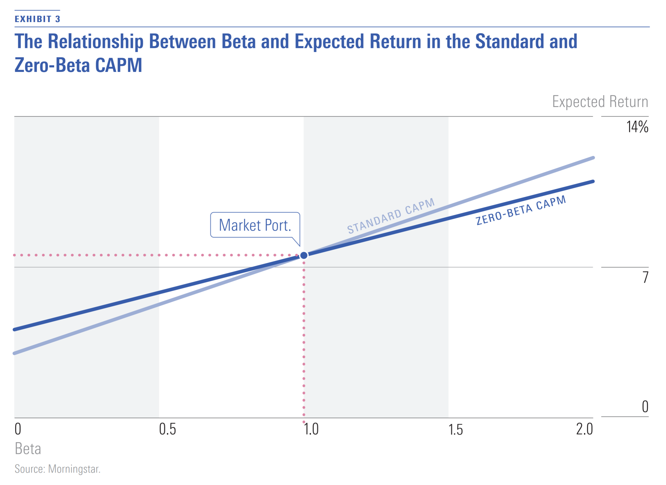
Empirically, many studies have shown that the relationship between beta and long-term average return (a proxy for expected return) is flatter than what is predicted by the standard CAPM. In other words, securities with low betas have higher average returns than predicted by the standard CAPM, and securities with high betas have lower average returns than predicted. The Zero-Beta CAPM provides one possible explanation for this. If the expected return on the Zero-Beta Portfolio is greater than the risk-free rate, as is the case in the example here, the line showing the relationship between beta and expected return is flatter than predicted by the standard CAPM.

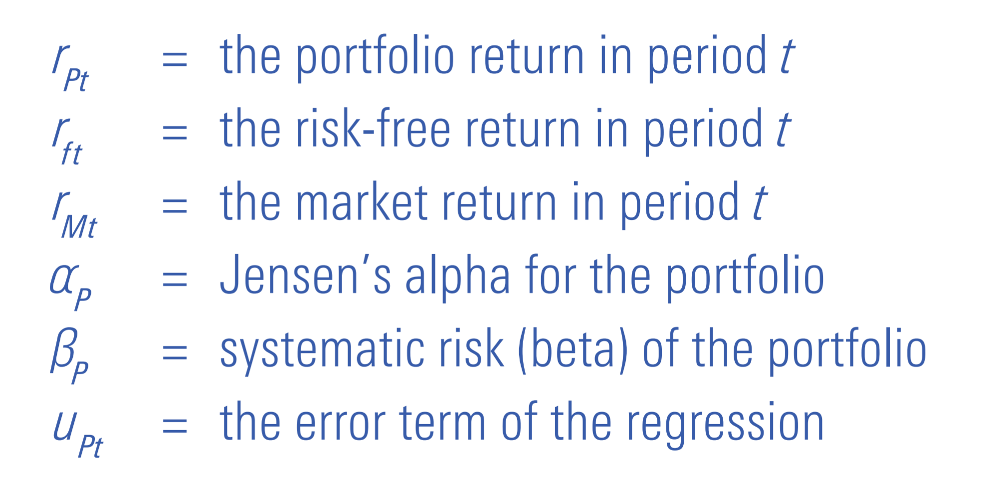
The flattening of the security market line has important implications for performance measurement. Jensen's alpha is a common measure of risk-adjusted performance of a portfolio or strategy. Jensen's alpha is usually estimated as the intercept in the following time-series regression:

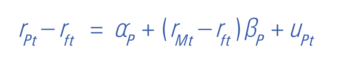
where:

If the standard CAPM does not hold, but the Zero-Beta CAPM does, the resulting flattening of the security market line in the absence of manager skill (positive or negative) induces positive alphas for low-beta strategies and negative alphas for high-beta strategies. Thus, the CAPM-based conventional alpha measure is biased up for low-beta strategies and biased down for high-beta strategies.

A Biased Measure The CAPM makes some very strong assumptions that lead to very strong conclusions. As I discussed in the Summer 2019 issue of Quant U, Markowitz (2005)[2] examined the implications of removing the assumption that investors can take short positions in any securities. Here, I discuss the implications of removing the assumption that investors can borrow and lend at the same riskless rate without limit, an idea first explored by Black (1972). One of the main implications of the resulting form of the CAPM, known as the Black CAPM or Zero-Beta CAPM, is the possibility that the security market line of the standard CAPM is too steep. This implies that Jensen's alpha is a biased measure of risk-adjusted return, favoring low-beta strategies and penalizing high-beta ones.

In the next issue of Quant U, I will discuss what happens when the assumption that all investors have the same expectations of security returns is removed, allowing for different investors to hold different views.

[1] Black, F. 1972. "Capital Market Equilibrium With Restricted Borrowing." Journal of Business, Vol. 45, No. 3, P. 444.

[2] Markowitz, H.M. 2005. “Market Efficiency: A Theoretical Distinction and So What?” Financial Analysts Journal, Vol. 61, No. 5, P. 17